Implementing MCMC - Hamiltonian Monte Carlo
This post is about Hamiltonian Monte Carlo, an MCMC algorithm that builds on the Metropolis algorithm, but uses information about the geometry of the posterior to make better proposals. If you are unfamiliar with the Metropolis algorithm, check out the previous post in this series. We'll start by understanding how the algorithm works, what problems it solves, then finish up with a simple implementation.
If you would like to know more about Hamiltonian Monte Carlo I strongly recommend A Conceptual Introduction to Hamiltonian Monte Carlo by Michael Betancourt, from which I learnt many of the things I'm writing about here.
The need for better proposals
In the previous post we successfully applied the Random Walk Metropolis algorithm to a couple of different problems. Generating a proposal by adding normally distributed noise to the current location is very simple and easy to implement, so why would we want to do anything else?
To understand the answer, recall that MCMC algorithms return a sample, of size say, from the target distribution. This sample is correlated, which motivates the introduction of the effective sample size . The error in the Monte Carlo estimator decreases like , so we can interpret our correlated sample as having the utility of an independent sample of size . The goal therefore is to maximise the effective size with the available resources (time and compute). There are two ways to increase :
- We can increase the total number of samples, or
- We can decrease the correlation in the samples.
These two possibilities are somewhat in tension. Decreasing the correlation in the samples probably means doing more work per sample which means producing fewer samples in total. On the other, simple fast methods for generating proposals might result in high correlation, but allow for large samples to be produced because they can be run so quickly.
The Random Walk Metropolis algorithm falls into the latter category here. Sampling from a normal distribution to generate the proposal is fast, but it turns out will lead to correlated samples. The following example illustrates why this is the case. Consider this (unnormalised) probability density, that is concentrated in an annular region.
import numpy as np


class DonutPDF:
    def __init__(self, radius=3, sigma2=0.05):
        self.radius = radius
        self.sigma2 = sigma2

    def __call__(self, x):
        r = np.linalg.norm(x)
        return np.exp(-(r - self.radius) ** 2 / self.sigma2)
Let's reuse the implementation of Random Walk Metropolis from the last post and use it to draw samples from this density. First recall the proposal distribution which simply adds normally distributed noise to the previous sample
class NormalProposal:
    def __init__(self, scale):
        self.scale = scale

    def __call__(self, sample):
        jump = np.random.normal(
            scale=self.scale, size=sample.shape
        )
        return sample + jump
We combine this with the Metropolis algorithm which generates proposals and applies an accept / reject criterion based on the target density
def metropolis(target, initial, proposal, iterations=10_000):
    samples = [initial()]

    for _ in range(iterations):
        current = samples[-1]
        proposed = proposal(current)
        if np.random.random() < target(proposed) / target(current):
            samples.append(proposed)
        else:
            samples.append(current)

    return samples
We'll run two simulations with different scales in the proposal distribution.
target = DonutPDF()
samples05 = metropolis(target, lambda: np.array([3, 0]), NormalProposal(0.05))
samples1 = metropolis(target, lambda: np.array([3, 0]), NormalProposal(1))
We can see what's going on by animating the samplers. The underlying contour plot shows the target density
Using both small and large jumps to generate proposals results in highly correlated samples. In the former case, each proposal is not very different from the previous sample so progress through parameter space is slow. In the latter case, there is a high probability the jump lands us outside the annular region where the probability density is vanishingly small, which means there is a high probability that sample is rejected. When a sample is rejected the previous sample is repeated, which results in high correlation in the samples, and hence small .
Furthermore, we haven't fully explored the target density. Neither sample makes it all of the way around the annulus, and both end up having their samples concentrated in a small sector.
What we ideally would like is a method for generating proposals that would result in less correlation in the samples, and better exploration of the target density. This is where Hamiltonian Monte Carlo comes in. But before we look at how it works, I want to quickly argue that this annular density example isn't completely contrived.
Consider a standard multivariate normal distribution . This is arguably the simplest high-dimensional probability distribution we might like to sample from. Let's look at how the distribution of distance to the origin in a sample changes as we increase the dimension.
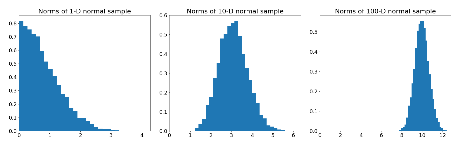
What we see from the histograms is that as the dimension increases, the samples become concentrated in an annular region further and further from the origin. Why does this happen? Well, remember that event probabilities are defined by integration
So the probability that a sample will land in region depends both on the density in that region, but also the volume of that region . Mass, including probability mass, depends on both density and volume.
The normal density is always largest at the origin in any dimension, but in higher dimensions there is much more volume away from the origin than there is near the origin, which means the product of and is maximised in the annular region. High dimensional spaces are weird...
The practical implication of this trade-off between volume and density, is that in high dimensions most of the probability mass is concentrated along narrow submanifolds, which are easy to fall off if we generate proposals with a random walk. To ensure the Markov Chain remains in the high probability mass region we need to use information about the density in our proposal distribution.
Hamiltonian Monte Carlo
Hamiltonian Monte Carlo uses ideas from Hamiltonian mechanics to generate a proposal by moving through parameter space according to a carefully constructed Hamiltonian system.
Here's some not terribly rigorous intuition. Imagine the graph of the negative log target density over parameter space. The high density regions of the target correspond to "wells" and "valleys" on this surface. Now imagine a particle released on the surface. It will roll "downhill" into the high density regions. If instead of simply releasing the particle we were to give it an initial push in a randomly chosen direction, it will roll around the surface, always being attracted towards high density regions, but sometimes having enough momentum that it rolls out into a lower density region, only to eventually slow down and return to the high density regions. If we construct the path that this imaginary particle would take, we can follow the path for a fixed amount of time, and then use the place we end up as the proposal in the Metropolis algorithm. That is, in essence, the Hamiltonian Monte Carlo algorithm.
Let's try and make that slightly more rigorous. I'm going to change notation here to be consistent with the standard notation in Hamiltonian mechanics. We'll denote by the parameters, which take the role of generalised coordinates in the Hamiltonian system, the target distribution, and the conjugate momenta. Together, defines phase space, expanding the -dimensional parameter space into a -dimensional space.
We will contstruct a Markov chain in phase space. To do so, we need to introduce a probability distribution over phase space. Since we ultimately want to recover a sample from the original target distribution , it's important that the marginal distribution of over is simply . For this reason we define the distribution over phase space by specifying the conditional distribution of given
which guarantees that is indeed the marginal distribution. We define the Hamiltonian as
which decomposes into two terms:
- The first, , is the negative log target density and can be thought of as the "potential energy" in the system. In the hand-wavey geometric picture from before, it is the height of the particle on the surface. As the particle rolls down into higher density regions this term decreases.
- The second, , can be thought of as kinetic energy. Unlike the first term which is determined by the target, we have full freedom to choose the form of this term.
A common choice for is a multivariate normal distribution
where is known as the mass-matrix. We have freedom to choose an arbitrary , so we would ideally make a choice that makes sampling as easy as possible. As it turns out, setting to be the inverse of the covariance matrix of the parameters is equivalent to transforming parameter space in order to maximally decorrelate the parameters, which helps sampling. Hence we set
Of course, this quantity is not generally known as is unknown. In practice, this covariance matrix is estimated from the samples in a warm-up phase, and the mass matrix is then updated for later samples. With estimated, we have
Since we are able to work with unnormalised densities, we can drop constants that are independent of and .
Evolving the Hamiltonian system
Hamilton's equations tell us how the system evolves in phase space. We have
Given a sample (I'm switching to indexing samples with to avoid a notation clash with the time evolution of the Hamiltonian system), we set and sample , we then evolve for a fixed time to obtain a proposal , which we apply the standard Metropolis acceptance criterion to. If we accept then we have , otherwise we stay where we are and set .
So how do we obtain ? We need to numerically solve the system. Many numerical solvers suffer from errors that compound over time, meaning that our estimate of gets worse as gets large. Fortunately, we can exploit the structure of the Hamiltonian system. Hamiltonian dynamics preserve phase space volume, which can be seen for example by observing that the vector field induced by Hamilton's equations has zero divergence.
A certain class of numerical approximation schemes - known as symplectic integrators - exactly preserve phase space volume, despite being discretised approximations. This limits the extent to which errors can accumulate, because for example diverging to infinity or spiraling to zero would typically require that the volume expands or contracts respectively. In particular, unlike naive schemes, errors do not compound, which allows us to approximate longer trajectories without the error becoming unacceptably large.
A simple and often used symplectic integrator is the so called leapfrog integrator. This sees us make a half step with , using the half-updated to update , then taking another half step with using the updated . In other words
We can test this with an extremely simple Hamiltonian
The figure below compares the leapfrog approximator to Euler's method and a modified Euler's method (see the appendix at the end of this post for details). The analytic solution is shown in grey. We see that Euler's method diverges completely. The modified Euler doesn't diverge as it is volume preserving, but does deviate from the analytic solution at times more than the leapfrog integrator, while the leapfrog integrator's trajectory is very difficult to distinguish from the analytic solution.
The reason the leapfrog integrator performs better than the modified Euler method is because in addition to being volume preserving it is also reversible, which implies better asymptotics for the global error rate in terms of step size.
Implementing Hamiltonian Monte Carlo
We have everything we need to implement Hamiltonian Monte Carlo. The algorithm is as follows:
- Choose a starting point in parameter space, and fix a step size and a path length .
- Given parameters we sample . More generally we could sample from where . We will however keep things simple and just use the identity matrix.
- We set . Evolve for steps using the leapfrog integrator to obtain , an approximation of .
- Sample and let if , or otherwise.
- Repeat
Ok, here goes. First the leapfrog integrator. As before, all implementations are optimised for clarity and simplicity rather than performance.
def leapfrog(q0, p0, target, L, step_size):
    q = q0.copy()
    p = p0.copy()

    for i in range(L):
        p += target.grad_log_density(q) * step_size / 2
        q += p * step_size
        p += target.grad_log_density(q) * step_size / 2

    return q, p
We then use that to generate proposals in the Metropolis algorithm. Note we slightly modify the implementation of Metropolis from before since we must compare ratios of the joint distribution over parameters and momenta rather than the target distribution.
def hmc(target, initial, iterations=10_000, L=50, step_size=0.1):
    samples = [initial()]

    for _ in range(iterations):
        q0 = samples[-1]
        p0 = np.random.standard_normal(size=q0.size)

        qL, pL = leapfrog(q0, p0, target, L, step_size)

        h0 = -target.log_density(q0) + (p0 * p0).sum() / 2
        h = -target.log_density(qL) + (pL * pL).sum() / 2
        log_accept_ratio = h0 - h

        if np.random.random() < np.exp(log_accept_ratio):
            samples.append(qL)
        else:
            samples.append(q0)

    return samples
We also slightly redesign the target, as we require evaluations of the gradient of the log density of the target. In this example I've hard-coded the gradient, but proper implementations typically use some form of autodiff to calculate gradients.
class DonutPDF:
    def __init__(self, radius=3, sigma2=0.05):
        self.radius = radius
        self.sigma2 = sigma2

    def log_density(self, x):
        r = np.linalg.norm(x)
        return -(r - self.radius) ** 2 / self.sigma2

    def grad_log_density(self, x):
        r = np.linalg.norm(x)
        if r == 0:
            return np.zeros_like(x)
        return 2 * x * (self.radius / r - 1) / self.sigma2
We can then draw samples
hmc_samples = hmc(DonutPDF(), lambda: np.array([3, 0.]));
The below animation shows what's going on. On each iteration we compute the trajectory according to the Hamiltonian system, then after a fixed time we stop and use the end point as a proposal in the Metropolis algorithm. In the animation, the trajectory flashes green or red depending on whether the proposal is accepted or rejected respectively.
We see that not only is the acceptance rate very high, but also the Markov chain quickly finds its way around the donut and covers parameter space quite evenly. The combination of a high acceptance rate and the potential to take large steps will result in a low auto-correlation and hence higher effective sample size.
Of course, calculating the trajectories of the Hamiltonian system at each time step is significantly more computationally expensive than generating a proposal by adding normally distributed noise. However, in practice it often turns out that the decrease in auto-correlation in the samples far outweighs the reduction in the number of samples, so we still get a better effective sample size which is a much better measure of the quality of our sample than the raw sample size.
Let's finish up by comparing the two Random Walk Metropolis algorithms with different scales from earlier to Hamiltonian Monte Carlo.
Even for this simple example the results are pretty striking. Random Walk Metropolis with small jumps makes small and limited progress around the donut in the first 1000 samples. With a larger jump size it manages to make it all the way round, but the acceptance rate is low and the samples are not very evenly spread. Finally Hamiltonian Monte Carlo achieves an extremely high acceptance rate and has very good coverage of the distribution. Even without calculating anything it's pretty clear that the sample from Hamiltonian Monte Carlo is the highest quality of the three.
Summary
The effective sample size is a good measure of the quality of a sample from a MCMC sampler. We can increase the effective sample size by either drawing more samples, or decreasing the auto-correlation in the samples. Random-Walk Metropolis which we saw in the first post is able to draw a large number of samples very quickly, but struggles to make good proposals as the dimension of parameter space increases: either it moves through parameter space very slowly or the proposals have a low acceptance rate. In either case the auto-correlation in the sample is high.
Hamiltonian Monte Carlo defines flows through parameter space along which the sampler travels to generate new proposals. This means the sampler can step further away from the previous sample while retaining a high acceptance probability. Each sample is more computationally expensive as a result, but we frequently see enough of a reduction in the auto-correlation in the sample for the trade-off to be worthwhile.
One thing we didn't discuss was how to choose the integration time , or equivalently in the approximation the step size and the number of steps . If we choose to be too large we might incur unacceptably large error, but too small and the exploration of parameter space will be very slow. Similarly if is too small we won't move very far through parameter space, but too large and we incur a large computational cost computing the flow, some of which may be wasted if the sampler covers old ground (imagine in the donut picture we do multiple laps before making a proposal).
There is no general combination of and that will work for all problems, because what a suitable value is depends on the target. Even worse, Hamiltonian Monte Carlo has been found to be quite sensitive to these parameter choices, and a bad choice can destroy the utility of the sampler. In the next post we will look at the No U-Turn Sampler (NUTS), a modification of Hamiltonian Monte Carlo that is able to choose appropriate and automatically, making it much easier to apply in practice.
Full code for all of the plots and animations in this post is available in this Gist.
Appendix
When introducing the leapfrog integrator we compared to two other approximation schemes, the details of which are as follows. First Euler's method. Given a step size we produce sequences of approximations and via the recurrence relations
As we saw this method can accumulate error leading to divergence. A modification to Euler's method sees us instead update using the updated value
This method is volume preserving, which results in much better guarantees on the error rate. The leapfrog integrator takes this one step further and partially updates , uses the partial update to update , then completes the update of with the updated . This modification adds a symmetry which ensures reversibility and further improves the error bounds.