Implementing MCMC - the Metropolis algorithm
I'm a big fan of probabilistic modelling and Bayesian inference. In fact at the time of writing that's the only topic I've written about on this blog so perhaps that's blindingly obvious... If you've ever dipped a toe into these warm waters then you'll likely have come across Markov Chain Monte Carlo (MCMC) algorithms. They are one of the workhorses of Bayesian inference, being an efficient, general purpose way to draw samples from a probability distribution. In this series of posts I want to develop some intution for MCMC algorithms by implementing them and applying them to a toy problem. In this post we'll understand the need for MCMC algorithms and learn about the Metropolis algorithm, the original MCMC algorithm and the foundation for many more advanced algorithms that were developed later. Let's get started!
What problem are we solving?
If you've not really worked with MCMC algorithms before, it might not be immediately obvious why we're so interested in drawing samples from a probability distribution in the first place. To understand why, let's take a step back and consider what problem we're actually trying to solve. Imagine we have a probability distribution over - characterised by density - about which we want to answer certain questions.
Note that I'm (semi-)implicitly assuming to be modelled by a continuous probability distribution here, so that we integrate over against . This is primarily for notational convenience at this stage, we could consider an arbitrary probability distribution characterised by probability measure in which case we can integrate directly against . In a later post, when we get on to the topic of Hamiltonian Monte Carlo, we will need to make some continuity assumptions.
Essentially every quantity that we might be interested in to answer questions about this distribution can be characterised in terms of integrals. An obvious example would be the expected value of
and similarly variances or covariances are simply integrals also. Perhaps slightly less obviously, event probabilities can also be characterised as integrals, since they are the expected value of the indicator function of that event
If is scalar, quantiles such as the median can be characterised via integrals
So the problem of doing inference on a probability distribution reduces to evaluating integrals. What we would like is a general way to evaluate or approximate these integrals.
When we first learn about integration, the focus is usually on evaluating integrals analytically. In reality it isn't hard to construct examples where this isn't possible, even in one dimension. If we want to evaluate a high dimensional integral we often will have no choice but to numerically approximate it. So what are our options?
Approximating integrals
Many algorithms have been developed for approximating integrals, they can broadly be split into two categories: deterministic and stochastic approaches. We'll suppose that given some function we want to evaluate
Deterministic approaches
Deterministic approaches typically start with some kind of grid of points for , then approximate the integral with a weighted sum of evaluations of the integrand on the grid
Simpson's rule for example is a particular special case of this, but there are many variants. There are two big drawbacks to these deterministic approaches that mean we will ultimately be uninterested in using them for inference:
-
If we were to use a naïve strategy for choosing grid points, then the number of points required to reach some acceptable level of error increases exponentially with the dimension of the space we are integrating over. For example, if we were using a uniform grid, then in one dimension we might require points for an acceptable level of error. In two dimensions, to achieve the same "resolution" we would need a grid of points, and so on so that in dimensions we construct a grid of points. Deterministic evaluation of integrals quickly becomes intractable as a result. There are of course algorithms that try to solve such problems, using adaptive grids and other tricks, but they will mostly be more complicated and less general.
-
A second problem, which is particularly relevant in Bayesian inference, is that we need to evaluate the density , whereas typically we might only know the density up to a multiplicative constant. We will see shortly that MCMC methods don't have this problem, as they can proceed with an unnormalised form of the density.
The Monte Carlo approximation
The Monte Carlo approximation is a stochastic integral approximation. Given samples for we approximate
that is we average evaluations of on the samples . Note that unlike the deterministic approaches above, the approximation does not feature evaluations of . This is instead accounted for by the fact that samples will be concentrated where is large. As a result we can think of the samples as being like an adaptive grid, which places more grid points in regions that have more influence on the value of the integral.
From the Central Limit Theorem we can deduce that asymptotically as
from which we learn that the variance of the Monte Carlo estimator, or specifically the asymptotics thereof, are independent of the dimension of ! This remarkable fact is one of the key reasons that the Monte Carlo estimator is so powerful when it comes to estimating high dimensional integrals.
Drawing samples
It might seem like we just got a free lunch, which should make you suspicious. How did we manage to get rid of the exponential scaling just by introducing some stochasticity? In truth we didn't get rid of it, we've just traded one problem for another. Rather than approximating integrals we need to figure out how to draw independent samples from an arbitrary probability distribution. A naïve approach will have the same exponential scaling with dimension as the deterministic integral evaluation, so really we've just shifted the complexity into the drawing of samples.
An interesting observation however, which opens the door to MCMC algorithms is that the independence requirement can be relaxed. We can use correlated samples instead, but the variance in the estimator will decay slower than . In fact we can quantify the price we pay for not having independent samples. We introduce , the effective sample size, defined as
where are the lag- auto-correlations in the sample. It can be shown that the variance in the estimator decays like , and so in some sense our correlated samples are "as good as" independent samples.
Notice that the less correlated the samples, the larger , so when drawing samples we want to find a balance of drawing as many samples as possible (increasing ) with making sure that those samples are as uncorrelated as possible (reducing the denominator). Both of these things will increase , but they are likely to be in tension.
Markov chains
A Markov chain is a sequence of random variables, where each variable depends only on the previous variable. That is satisfies . As a result, Markov chains can be characterised by transition kernel , which represents the probability of transitioning from to in one step.
A classic example is that of a random walk, where . That is, at each time step we take a step in the direction which is drawn from some appropriate probability distribution like a multivariate normal distribution.
Markov chains have some nice convergence properties assuming certain conditions are satisfied. There's a lot of theory behind these results that I won't go into in detail in this post. The key thing to know is that under certain regularity conditions, the chain will have a so-called stationary distribution. The stationary distribution is unique, and invariant under the transition kernel. That means if we sample a starting point from the stationary distribution, then take a step according to the transition kernel, the result is also distributed according to the stationary distribution. Furthermore we have that the Markov chain will converge to that stationary distribution from any starting position.
The practical implication therefore is that if we can construct a Markov chain whose stationary distribution is the target distribution, then we know that samples from the chain will look more and more like samples from the target distribution if we evolve the chain for long enough. This is precisely what the Metropolis algorithm does.
The Metropolis algorithm
We want to construct a Markov chain whose stationary distribution is the target distribution. To do so we need two ingredients:
- The target probability distribution (which need not be normalised)
- A jumping / proposal distribution , which given the current location in parameter space , defines a probability distribution over possible locations at the next time step. The Metropolis algorithm requires that this proposal distribution is symmetric so that , i.e. the probability of jumping from A to B is the same as the probability of jumping from B back to A. This requirement can be relaxed.
The idea of the algorithm is to evolve the Markov chain by sampling a proposal from the proposal distribution, then applying an accept / reject criterion based on the target distribution that will ensure the chain as a whole has the correct stationary distribution. It is worth understanding this setup well, as many more advanced algorithms follow the same structure, they just use clever choices of .
The details are as follows:
- Choose a starting point .
- Given , sample from the proposal distribution .
- Sample . If , set , otherwise set .
- Repeat times.
The ratio represents how much more likely the proposal is under the target distribution than the current sample . If the proposal is in a region of higher density than the current sample it will always be accepted (because ), otherwise if the proposal would take the chain to a region of lower probability (under the target distribution), there is a non-zero chance the proposal is rejected and the chain stays where it is. A proof that this procedure results in the target distribution being the stationary distribution is included in the appendix at the end of this post.
Notice that because the target distribution only enters the algorithm in the form of this ratio, it is ok if we only know the target distribution up to a multiplicative constant independent of , as such constants will cancel out anyway. This is exactly the situation we find ourselves in when doing Bayesian inference. It's easy to specify the unnormalised prior as the product of the prior and the likelihood
Ordinarily the data marginal / evidence in the denominator is hard to calculate (it is itself defined in terms of an integral over ), but thanks to the Metropolis algorithm we needn't calculate it and can instead just work with the unnormalised product.
Implementing Metropolis
Let's have a go at implementing the Metropolis algorithm. To do so we'll need to specify a proposal distribution which we haven't discussed yet. One of the simplest, and perhaps most common, choices is a normal distribution
where is a tunable parameter. That is to say, at each step the proposal is simply the current sample with some normally distributed noise applied. This is very easy to implement, and is known as Random Walk Metropolis, as the proposal distribution is defining a random walk in parameter space.
Below is a simple implementation of the metropolis algorithm. It expects an
unnormalised density target corresponding to the target distribution, a
function initial that can produce an initial sample, and a proposal
distribution proposal that returns a sampled proposal given the current point.
The implementation could certainly be improved, I'm attempting to optimise for
clarity rather than anything else.
import numpy as np


def metropolis(target, initial, proposal, iterations=100_000):
    samples = [initial()]

    for _ in range(iterations):
        current = samples[-1]
        proposed = proposal(current)
        if np.random.random() < target(proposed) / target(current):
            samples.append(proposed)
        else:
            samples.append(current)

    return samples
You'll notice that the core logic of this algorithm is really very simple. Abstracting away the proposal it's only a handful of lines of code. Don't be fooled by the simplicity though, this basic structure can be extremely powerful.
Let's implement a proposal distribution. This can quite neatly be encapsulated
with a custom class which we make callable by implementing the __call__ magic
method.
class NormalProposal:
    def __init__(self, scale):
        self.scale = scale

    def __call__(self, sample):
        jump = np.random.normal(
            scale=self.scale, size=sample.shape
        )
        return sample + jump
Instantiating NormalProposal produces a callable object that adds normally
distributed noise with the specified scale to the argument.
We also need a target distribution to sample from. Let's start simple and use a multivariate normal distribution. Again, this can be quite neatly implemented as a callable object.
class MultivariateNormalPDF:
    def __init__(self, mean, variance):
        self.mean = mean
        self.variance = variance
        self.inv_variance = np.linalg.inv(self.variance)

    def __call__(self, sample):
        return np.exp(
            -0.5
            * (sample - self.mean).T
            @ self.inv_variance
            @ (sample - self.mean)
        )
Notice that this object returns an unnormalised form of the density, ordinarily there would be an additional factor depending on the determinant of the covariance matrix.
We can put this all together and draw samples
samples = metropolis(
    target=target,
    initial=lambda: np.array([0, 0]),
    proposal=NormalProposal(0.1),
    iterations=50_000,
)
I ran this four times with different starting points each time. The results are shown below
You can see from the animation that the early samples, when the chain is still finding its way to the high density region of the target distribution are not very representative of the target, however once the chains have found their way to the high density region they explore it fully and mix well.
Understanding when the chain has converged is one of the challenges of MCMC. Various diagnostic metrics have been introduced which I won't go into here. One basic idea that suggests itself when you look at the animation above is to run multiple chains and compare them after some samples have elapsed. In the simple example, the chains quickly become indistinguishable, suggesting (but not proving) that they have converged to the shared target. The metric provides a more rigourous quantification of this observation than the "eyeball metric" that we used.
Fitting Logistic regression with the Metropolis algorithm
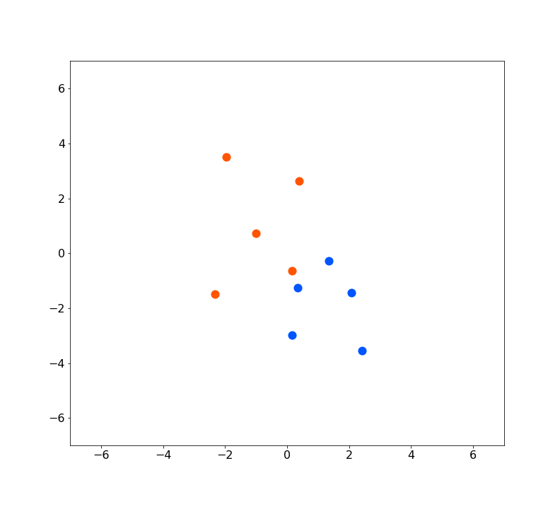
Sampling from a normal distribution is a little underwhelming. Let's finish up this post by trying something a bit more interesting. Let's generate some simple data for classification.
def sigmoid(arr):
    return 1 / (1 + np.exp(-arr))


alpha = -1.5
beta = np.array([1.5, -1.6])

data = np.random.multivariate_normal(
    np.zeros(2), np.array([[4, -2], [-2, 4]]), size=10
)
labels = np.random.binomial(1, p=sigmoid(data @ beta + alpha))
This gives us ten data points with five belonging to each class
Let's see if we can separate them with a logistic regression model. A standard setup would be something like the following
We want to sample from . Let
By Bayes rule we have
That looks easy enough to implement, so let's try it!
class LogisticPDF:
    def __init__(self, x, y, prior_scale=5):
        self.x = x
        self.y = y
        self.prior_scale = prior_scale

    @staticmethod
    def _likelihood(x, y, alpha, beta):
        eta = 1 / (1 + np.exp(-(alpha + np.dot(beta, x))))
        if y == 1:
            return eta
        return (1 - eta)


    def __call__(self, sample):
        alpha, beta = sample
        prior = np.exp(
            -(alpha ** 2 + np.linalg.norm(beta) ** 2) / (2 * self.prior_scale ** 2)
        )

        likelihood = 1
        for x, y in zip(self.x, self.y):
            likelihood *= self._likelihood(x, y, alpha, beta)

        return prior * likelihood
The way I've written this, each sample is a tuple consisting of an sample and a sample, so we also need to slightly rewrite the normal proposal from before.
class NormalProposalLogistic:
    def __init__(self, scale):
        self.scale = scale

    def __call__(self, sample):
        alpha, beta = sample
        alpha_jump = np.random.normal(
            scale=self.scale, size=alpha.shape
        )
        beta_jump = np.random.normal(
            scale=self.scale, size=beta.shape
        )
        return alpha + alpha_jump, beta + beta_jump
That's it, we can use the same metropolis function from before to draw samples
target = LogisticPDF(data, labels)
proposal = NormalProposalLogistic(0.1)
samples = metropolis(target, lambda: (np.array(0), np.array([0, 0])), proposal)
This gives us many samples of the coefficients in the model. The posterior predictive distribution is given by averaging the sampling distribution against the posterior.
In practice this means making a prediction with each sampled set of coefficients and then averaging the predictions. The result of doing this in our case (discarding the first 10,000 samples to minimise bias from the initialisation) is shown below.
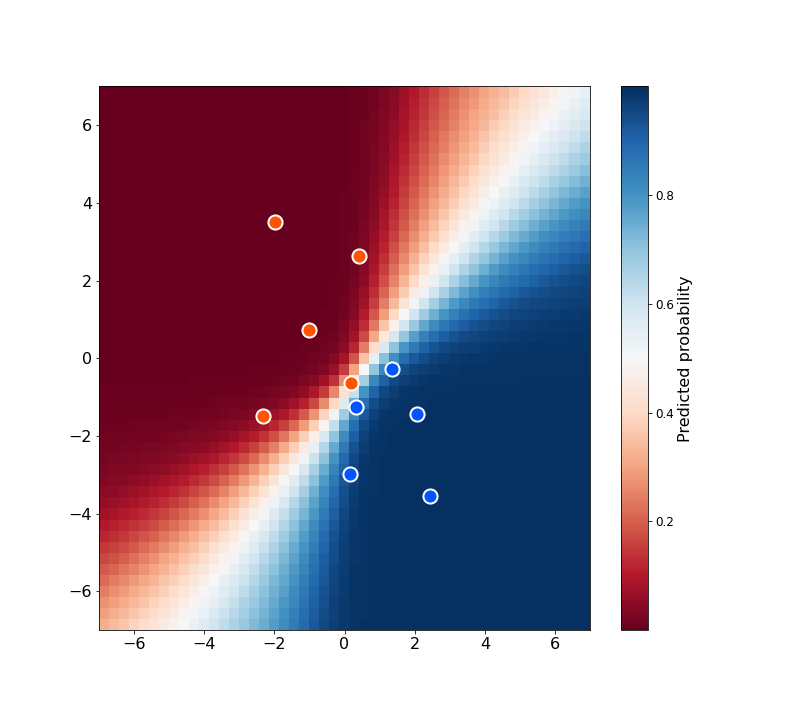
There we have it, a simple logistic regression solved by MCMC. From the heatmap you can see there is some uncertainty in the decision boundary, a consequence of the range of plausible parameters that could have given rise to the observed data. This is just one example of the benefits of inferring a distribution over parameters rather that simply a point estimate.
You'll notice that it was pretty easy to separate concerns in our implementation
of Metropolis. Once the core logic was in place (the metropolis function) we
were able to draw samples from a couple of different distributions just by
implementing a target density and a proposal distribution. The fact that we
don't have to normalise the target distribution helped make this very easy for
us. In the first example it would have been easy enough to implement a correctly
normalised multivariate normal density, but in the case of the logistic
regression it would have been at the very least annoying to do analytically. For
more complex models it's often impossible.
Conclusion
In this post we learned that statistical inference boils down to evaluating (often analytically intractable) integrals. We saw that the Monte Carlo estimator is a powerful stochastic integral approximator, which means to approximate integrals we can draw samples instead. Though drawing independent samples can be challenging, we learnt that correlated samples will do just fine, as long as we account for the amount of correlation in the sample when making inferences. The Metropolis algorithm is a general algorithm for sampling from any target distribution by constructing a Markov chain whose stationary distribution is the target distribution. We implemented the Metropolis algorithm and used it to sample from a multi-variate normal distribution, and to solve a simple logistic regression problem.
In the next post in this series, we're going to take a look at Hamiltonian Monte Carlo, which uses the geometry of the target distribution to construct a very efficient proposal distribution. We'll learn how it works and then try implementing it like we did here.
Full code for all of the plots and animations in this post is available here.
Appendix - stationarity of the target distribution
We show that the target distribution satisfies detailed balance with respect to the transition kernel induced by the Metropolis algorithm. Specifically, we want to show for any and we have
where is the transition kernel. Note that the transition kernel incorporates the accept / reject step and is not the same as the proposal distribution.
To prove this let's pick arbitrary and . Suppose , which we may do without loss of generality. Then the proposal will always be accepted from state so and hence
Going in the other direction, the proposal is accepted from state with probability , so using the fact that the proposal distribution is assumed to be symmetric
from which detailed balance follows, and hence the fact that is the stationary distribution of the Markov chain.